Results
Regression
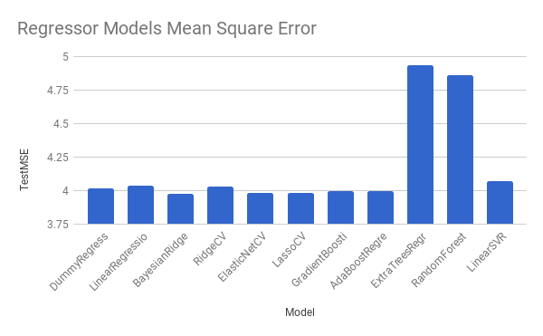
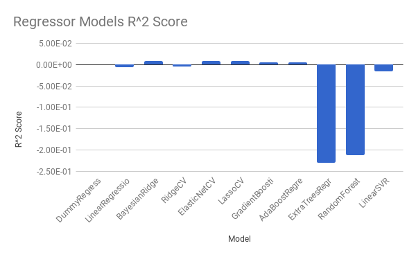
| Models | Duration | Train MSE | Test MSE | R2 Score |
|---|---|---|---|---|
| DummyRegressor | 0.0003519058 | 4.292656363 | 4.012747466 | -8.05E-06 |
| LinearRegression | 2.876500845 | 4.168436111 | 4.03817326 | -0.0063443617 |
| BayesianRidge | 9.113944054 | 4.240433111 | 3.978284211 | 0.0085804578 |
| RidgeCV | 14.15430808 | 4.167578924 | 4.03089686 | -0.0045310258 |
| ElasticNetCV | 6.157432079 | 4.24524836 | 3.981448748 | 0.0077918304 |
| LassoCV | 6.049508095 | 4.244920397 | 3.981493739 | 0.0077806182 |
| GradientBoostingRegressor | 10.3492372 | 4.250431632 | 3.994107012 | 0.004637292 |
| AdaBoostRegressor | 32.49189615 | 4.263147054 | 3.994472842 | 0.0045461242 |
| ExtraTreesRegressor | 70.33536506 | 0.2614326469 | 4.934085332 | -0.2296126575 |
| RandomForestRegressor | 135.7508721 | 1.08187359 | 4.861826425 | -0.2116051728 |
| LinearSVR | 53.98221612 | 4.314991285 | 4.073052891 | -0.0150366387 |
Most regressors actually have metrics quite similar to the DummyRegressor (a regressor that disregards the input and only outputs the mean target value). This shows that our ‘smart’ regressors are having trouble learning how any of the feature correlate to the plus/minus per minute target value.
There are two execptions out of the ‘smart’ regressors that attempted learning. We can see that the Tree-based Regressors (ExtraTressRegressor and RandomForestRegressor) perform fairly well when looking at only the training data metrics. They have a lower mean square error than the DummyRegressor. However, when evaluating these two models against a test dataset rather than a training dataset, both the mean square error and score show much worse results than all other regressors, including the DummyRegressor. This is certainly a sign of these models overfitting on the training data, and not learning the true relationship between the features and the target value.
Examining the Data
The poor results of the regression models can be attributed to issues in the models or data. A closer examination of the data indicates the latter due to a substantial amount of noise.
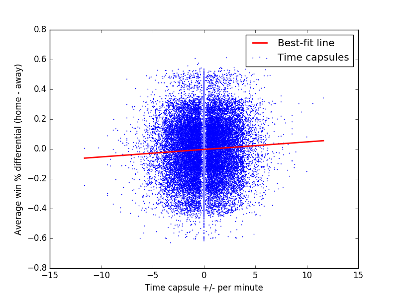
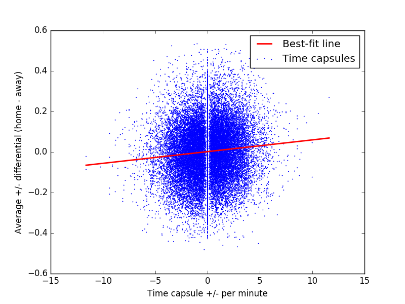
The scatter plots above help demonstrate this noise. Each point represents a time capsule, with the x-position indicating the plus-minus per minute for that capsule. For the y-position, we take the training data (which uses season-averaged player statistic), average the five home and five away team players’ statistics for each time capsule, and compute the difference in a statistic. We would expect teams with a high win percentage to outscore opponents with a low win percentage. From the best fit line, we can see this is roughly true, but the correlation between plus/minus per minute and win percentage is almost zero. A similar situation occurs when we compare time capsule plus/minus per minute to season-averaged plus/minus per minute.
There are several reasons we have hypothesized as to why this noise is present
- Time capsules are as short as 30 seconds. This does not allow must time for scoring to “smooth out” like it would over an entire game.
- Scoring streaks cause a large number of outliers.
- If a team is winning by a large margin at the end of a game, they may allow opponents to score more since it will not affect the game outcome.
These results suggest that a classification model might perform better, as it simplifies the problem.
Classification
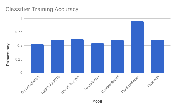
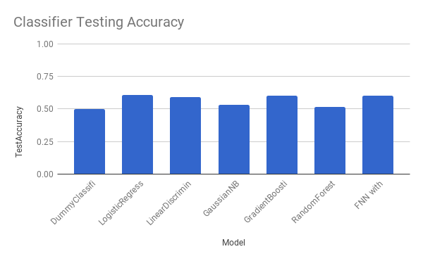
| Models | Duration | Train Accuracy | Test Accuracy |
|---|---|---|---|
| DummyClassifier | 0.001994133 | 52.14% | 49.71% |
| LogisticRegression | 8.462990046 | 60.50% | 60.58% |
| LinearDiscriminantAnalysis | 6.796962977 | 61.12% | 58.98% |
| GaussianNB | 0.6752369404 | 53.71% | 53.22% |
| GradientBoostingClassifier | 147.259727 | 60.08% | 60.31% |
| RandomForestClassifier | 5.883100033 | 94.39% | 51.62% |
| FNN with Dropout Reg | 46.352 | 60.65% | 60.36% |
Modifying our approach to a classification problem lets us train models that produce more meaningful results than the regression models. Just like the previous approach, we can compare the smart models against a DummyClassifier, which only outputs the most common label. We find all of our models perform at least as well as the DummyClassifier in terms of accuracy. LogisticRegression, GradientBoostingClassifier, and FFN with Dropout even reach 60% accuracy while the DummyClassifier performs as well as a coin flip.
Comparison to Previous Work
Torres et. al. and Loeffelholz et. al. both attempted to predict results of NBA games using machine learning.1 2 They used box scores of teams from games played earlier in the season to train their models then they used the trained models to make predictions about the remaining games in the season. Below is a table showing the results from both experiments:
| Source | Model | Average Classification Accuracy |
|---|---|---|
| Loeffelholz et. al. | FFNN | 71.67% |
| RBF | 68.67% | |
| PNN | 71.33% | |
| GRNN | 71.33% | |
| PNN Fusion | 71.67% | |
| Bayes Fusion | 71.67% | |
| Torres et. al. | Linear Regression | 69.91% |
| Logistic Regression | 67.44% | |
| SVM | 65.96% | |
| ANN | 64.78% |
Comparing the results from the table above with the results from our models, we can see that our models do a descent job of making predictions given that we are solving a harder problem of predicting results given player matchups rather than learning team performance over different games and seasons. Also, our model tries to select the best players to give a team the best chance of winning, and it learns by examining player statistics from a 30-second time capsules over a season. This presents a significant challenge even for a human expert.